ray tracing
an ode to rendering
May 25, 2025
Table of Contents
- Introduction
- The Beginning
- Fundamentals
- Cameras
- Spheres
- Materials
- Light
- Implementation
- oh im too lazy to read bring me to the end
- Formalization
Introduction
what are we talking about?
Back in 2018, NVIDIA released the RTX 20 turing series. 7 years later, NVIDIA has released the 50 series lovelace series of cards. NVIDIA is also one of the most valuable companies in the world now, interchangable with Apple. Today, NVIDIA sells their GPUs as professional AI cards, eating away hundreds of GB of memory to run and train gigantic LLMs. The GPUs have too many tensor cores for all the matmuls. But back when they were first released, RT cores headlined with the tensor cores [which were also partially designed for ray tracing!]—specialized hardware units which is more or less an ASIC for specialized ray tracing instructions.
It’s 2025 now, and I think there are still more games being released that are “RTX ON” but nobody really cares anymore. Maybe it’s cool how normal that is. Game engines [looking at you UE5] look so good these days it’s pretty insane. Ray tracing is far more than that, but that’s what got me interested. It’s used intensely in CGI, and excels in reproducing photorealistic scenes that older methods could not hope to achieve.
I do not believe this article is a better introduction to ray tracing than say, Shirley’s Ray Tracing in a Weekend. If you are interested in building ray tracers and hacking on them, that is likely superior. I hope to share some of my intuitions that’s slightly more rigorous with less emphasis on the code. However, since the theory of ray tracing is designed to end up implemented, a code heavy introduction may be better. But that’s not going to stop me from writing this.
The Beginning
why do I care?
It’s cool. That’s all. 2021 summer I didn’t really know what to do. I spent COVID–19 grinding out some codeforces [quite possibly one of the best investments I have ever made] but for whatever reason didn’t want to keep doing it. At least not as much as learning something new. This ray tracing thing was pretty cool—and I had come across Peter Shirley’s article. Ray Tracing in a Weekend.
I read it, I followed along line by line, and I made something… acceptable. It was clunky, unergonomic, definitely not performant, C++ code. You can find it here if you really want. It’s not even organized like a project. But it was lovely to me nonetheless. I spent a few weeks that August tinkering with this silly thing. And it worked!
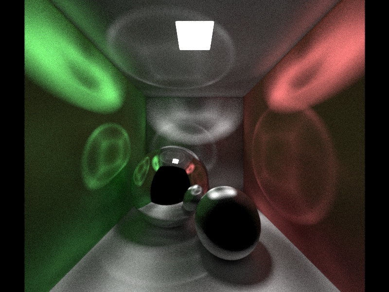
this is wrong but it looks pretty cool!
I played around with it some more, giving it multithreaded support [in totally the wrong way] - but it ran fast enough to give me a little animation. Although this took like a day to render on an M1 air.
cool gif right? cornell admissions didn’t agree though
My senior year of high school started. I don’t remember that much to be honest, but I do remember being in AP Bio [shoutout Mrs. Caveny + bradomination] and doing jack in the back of class. I mean I’d do the work and answer whatever questions and get like 70% on the homework quizzes, but during class [lecture?] I’d sit in the back of class and hack on a new ray tracer [to my credit I always finished tests first and got 100s].
After writing my first ray tracer in a scattered like 15 files of C++, I decided it would be fun to write it in the most minimal way. So I wrote it in C. The full implementation is around 500 lines of C code - much cleaner [not good C code but good effort from a high schooler!]. And much faster. I don’t have the exact measurements but I remember being able to render on the order of a single thread running in C [bc I didn’t know how to use pthreads] being roughly equivalent if not faster to 10 threads in whatever 6 + 2 configuration the M1 has.
So, I’d work on that little thing, maybe a little too much. Before long, I was done. And I then wondered - how could I go even faster? More cores! What has a lot of cores? The GPU.
As an ignorant high schooler [because I am slightly less ignorant now], I did not know how OpenGL worked. I thought it was solely for rasterization, and thus did not think I could use it for ray tracing. A few stackexchange posts also agreed with that sentiment, which settled it. See shadertoy for blatant proof otherwise. Today, ChatGPT would probably save my ass here. But regardless, I had to settle for another option. I used OpenCL, which is a much more full fledged computing language. I spent around a month, at least according to the git commits, learning OpenCL and how to invoke kernels from C. Fun process! And of course, I wanted it to be interactive because GPUs are for gaming after all. Thus, I needed a window to display my beautifully ray traced output. But the window used OpenGL! So, the flow of data went like the following:
CPU (C) -> GPU (OpenCL) -> CPU (C) -> GPU (OpenGL). This is pretty awful, and the last two data transfers could be cut out entirely had I known this could all be done in OpenGL. But it was fun! And maybe that’s all that’s important.
I had some mishaps on the OpenCL side, and honestly still do. My glass material doesn’t work fully for some reason, and I’m not particularly interested in debugging it. It will stain it for the rest of time I suppose.
“real time” ray tracing!
After this ray tracer, I let it off for a while. I didn’t really know what else to do, and it was college application season anyways. Not that I used the time on college applications.
A year and a half later in 2023, I took a class that was introduction to ray tracing. It went through the first Shirley article and touched on the second. I knew I wasn’t going to learn anything in this class but that didn’t stop me from taking it. The class was in effect, an excuse for me to spend 2 months thinking about ray tracing, reading about it, and absolutely sweating the living hell out of my final project. So I did. That’s literally what I did. I downloaded Veach’s thesis. I downloaded papers. I finally pulled out the second edition of PBRT that I bought back in 2022. Hundreds of pages of papers and thousands of lines of code later, I could render the following image:
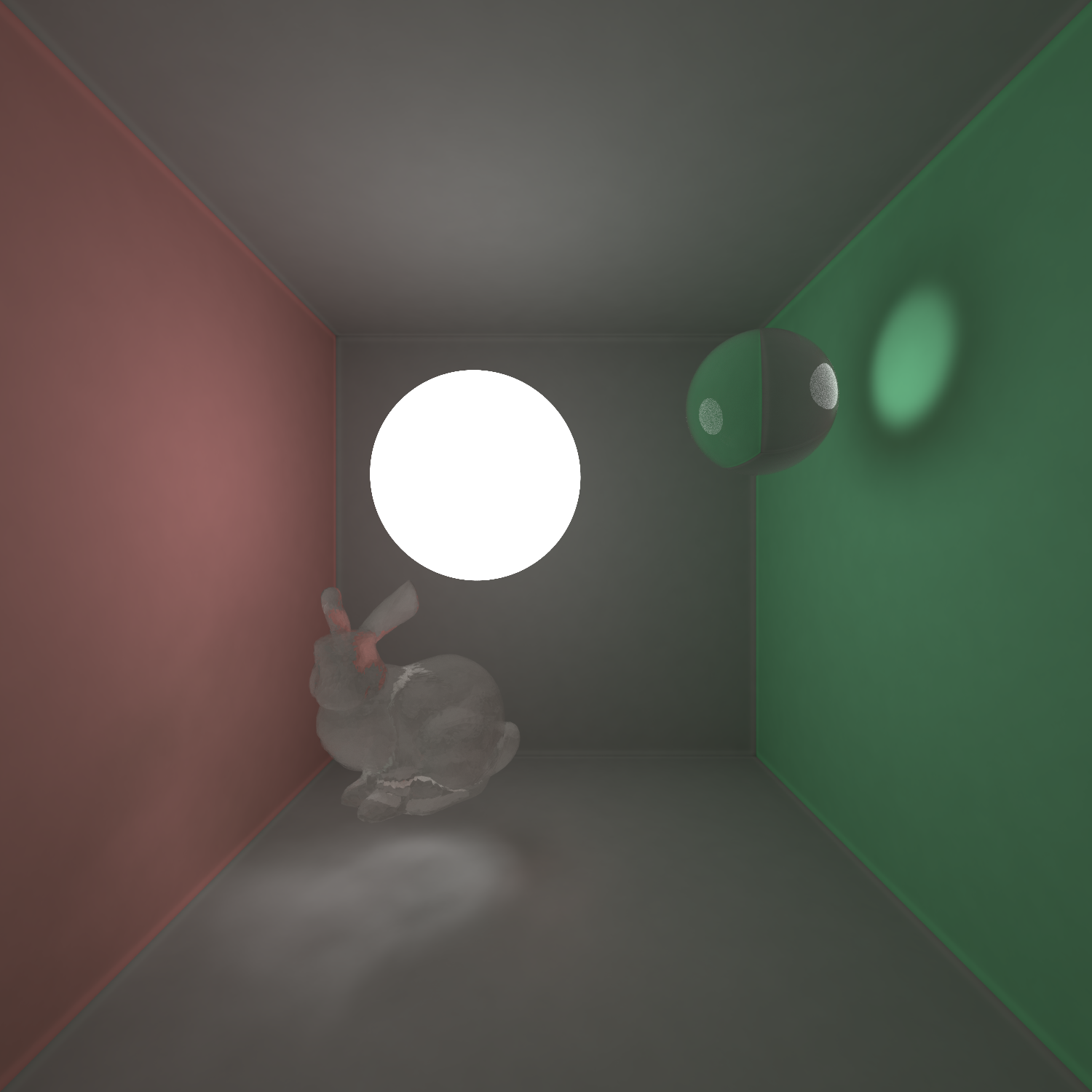
cool glass rabbit! nice reflections and details! there’s a better picture on my website’s homepage
The most recent one was December 2023—my compilers class was in OCaml, so I wrote a ray tracer in OCaml. I’m basically Matt Godbolt at this point.
It’s a pretty cool subject, and here’s an exceptionally fast paced introduction to it.
Fundamentals
ok ryan “phd in yapology” zhu. so how do I actually do anything?
The premise of ray tracing is to simulate light [gee why didn’t I think of that?]. While I don’t understand very much physics, we model it as a particle that is emitted from a light source, bouncing off surfaces [losing energy in the process and gaining “color”] before reaching the eye [camera]. We are interested in simulating this entire process.
Concretely, we simulate light as a ray with an origin and a direction $(\mathbf{o}, \vec{d})$ in 3D space. Light travels indefinitely until it hits a surface, where the material of the surface determines how light reflects off of it.
Some more terminology - the ray can intersect the plane at an angle, and the outwards pointing [outwards is defined by the object] direction in which the surface is facing is called the normal, denoted $\vec{n}$. We’ll call the incoming ray $\vec{\omega_i}$, and the outgoing ray [as a result of this reflection] as $\vec{\omega_o}$.
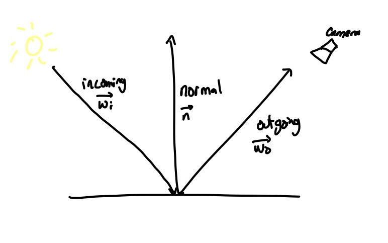
apologies for the handwriting in advance. you’ll have to get used to it.
Question: when light is emitted from a source, what’s the probability it ends up hitting the camera?
Answer: I don’t know. But probably pretty small.
Nuanced answer: It depends on the scene.
in many scenes, the probability of a random ray of light hitting the camera is exceptionally small
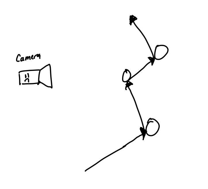
We invert the ray tracing process—so instead of tracing from sources to the camera, we’ll trace from the camera to the source. This inverts what we’re looking for. Instead of hoping the rays hit the camera, we’ll hope they hit a light source. Usually, this is easier! How much does this change in how we plan to simulate light? Not much really. Since we’re modeling simple materials, there are no pathlogical cases for us to consider.
Then, we’ll be tracing simulating light rays in reverse from the camera into the scene, letting them bounce, and recording the color of each pixel to construct an image. Sounds simple enough!
for the sections below, assume all vectors are unit vectors unless otherwise said
Cameras
if you’re an expert, what does ISO stand for?
Cameras are a funky business and we in effect must simulate a camera to render our scenes. We’ll make it easy and only consider a stupid simple perspective camera made up entirely of a pinhole sensor. I personally have never really looked into more complex camera setups—if I ever get to it I’d be happy to talk more about it.
For our purposes, a sensor is going to be a $n \times m$ array of pixels. Thus, we want to know what color each pixel on this grid will be, and to do so we will be tracing rays through each pixel out into the scene, in hopes some light will be hit. We will need to know the field of view [how much of the scene in front of us will be traced onto the sensor] and the orientation of the camera. Technically, this will be an angle degree $\theta$ for the angle swept out by the camera, as well as a triplet of vectors for the camera’s position, forward direction, and up direction, which we’ll call $(\mathbf{o}_c, \vec{d}_c, \vec{u}_c)$ respectively. Note that we cannot lack of any of these, as otherwise we wouldn’t know where to trace rays from and to.
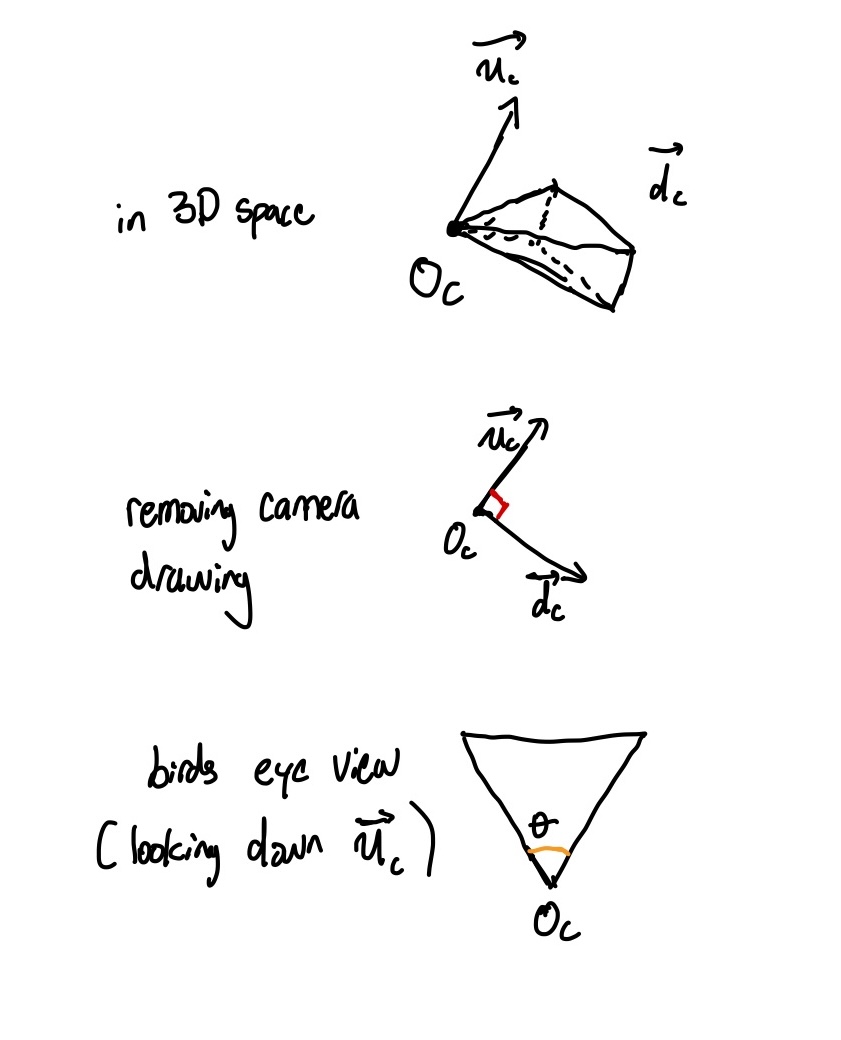
diagram of camera rays
Introduced Symbols
- $\theta$: horizontal FOV of the camera
- $\mathbf{o}_c$: origin position of the camera
- $\vec{d}_c$: forward direction of the camera
- $\vec{u}_c$: upwards direction of the camera
We’ll now go through the necessary technical details to implement our camera.
The main goal of the camera is twofold: to contain the sensor pixels and accumulate the color at each pixel, and to tell us how to trace rays out of the camera into the scene.
As an interface, we will at the very least need something along the lines of the following functions:
get_color(row, column) -> color accumulated at (row, column) [no side effects]
add_sample(row, column, color) -> void [side effect is to accumulate that color]
get_ray(row, column) -> ray representing a ray traced from the camera origin through the pixel at (row, column) [no side effects]
The first two functions are relatively simple - if we maintain a grid of colors, this is more or less just a getter and setter. The last function is the tricky one, and will require some effort.
If we can find calculate the center of each pixel as $\mathbf{o}_{rc}$, get_ray(r, c) will return rays that look like $(\mathbf{o}_c, \mathbf{\hat{d}}_p)$ where $\mathbf{\hat{d}}_p = \frac{\mathbf{o}_{rc} - \mathbf{o}_c}{\Vert\mathbf{o}_{rc} - \mathbf{o}_c \Vert}$—in English, this returns the ray that originates at the origin of the camera, and points at the center of the given pixel with a normalized direction.
How do we calculate the center of each pixel? Since we know the FOV of the camera, we consider a grid projected in the direction given by $\vec{d}_c$ in the ‘pyramid’ swept out by $\theta.$ We’ll imagine the grid to be exactly one unit vector away for the basis for our directions. Then, we can draw a triangle and solve for the distance of half the width by solving $w/2 = \tan(\theta/2).$ Then, we see that the width of a pixel can be $w/n$, where $n$ is the number of pixels on the width. Let’s call this length $l_p$, for the side length of a pixel.
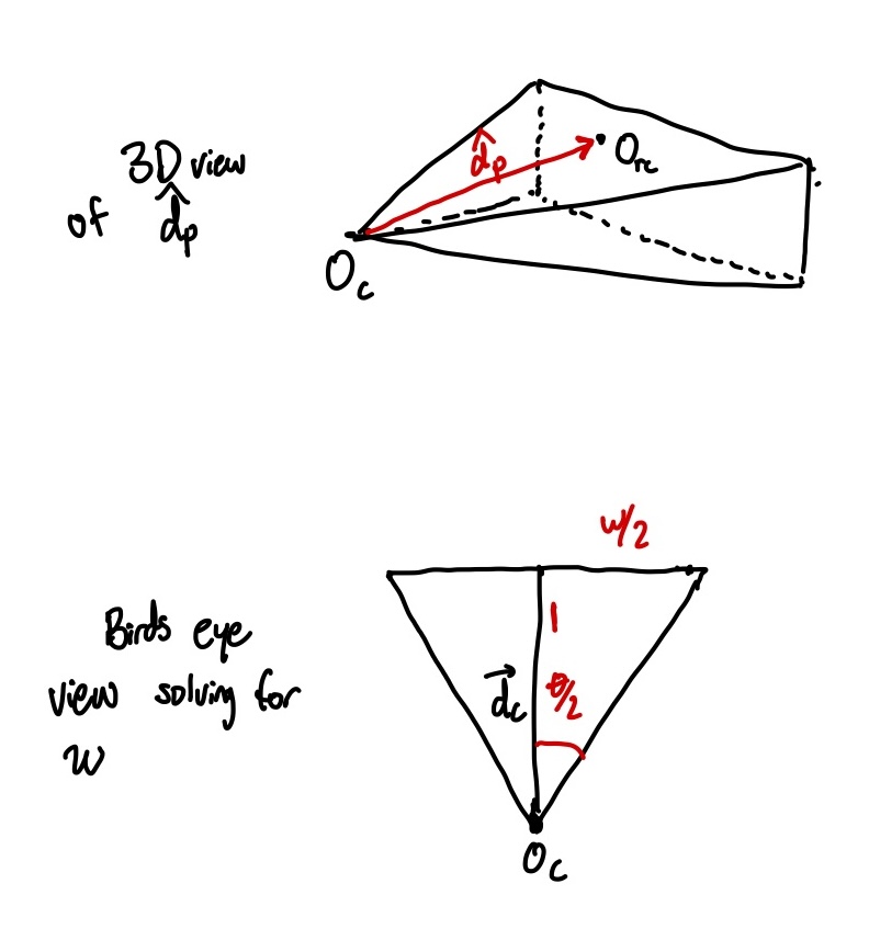
$\mathbf{\hat{d}}_p$ and solving for $w$
Question: But Ryan, what grid is this? Is the corner of the triangle on a pixel center? Shouldn’t we adjust by $n–1$ as the fencepost problem?
Answer: Probably? But this barely matters. How do you want to fix the even/odd debacle? Switch on the case and have perfect alignment? This is doable but to me not worth it.
Answer 2: Since the width is usually over 100 pixels, I don’t mind a drift of $< 1\%$ on the sensor. Since we are doing graphics for pretty pictures, this is okay. If you want precise images and simulations, think a little harder. [if this is unacceptable let me know with an argument and I’ll fix it]
Now with the width of a pixel [and height, since these are squares], we can go and find the midpoint of any pixel. For simplicity, let’s assume that $\mathbf{o}_c + \vec{d}_c$ points exactly at the rounded down middle pixel center. We can calculate every center by subtracing the width and height enough times. But we haven’t calculated the right/left vector yet! Not to worry, we can simply take the cross product $\vec{d}_c \times \vec{u}_c$ to give us the rightward direction [relative to the grid] which we can call $\vec{r}_c$. Then, to move 10 pixels to the right and 10 pixels down from the center we can do $$\mathbf{o}_c + \vec{d}_c + 10l_p * \vec{r}_c – 10l_p * \vec{u}_c.$$ Clearly, we could go ahead and store all the centers of the pixels. But this is unnecessary, and we’ll trade the $n \times m$ vector for some cheap arithmetic whenever we call get_ray. if we let the bottom left pixel be pixel $(0,0)$, then we can simply store that pixel as $\mathbf{o}_{bl}$ and we will have the following: $$\text{get_ray}(r,c) = (\mathbf{o}_c, \mathbf{o}_{bl} + r * l_p * \vec{r}_c + c * l_p * \vec{u}_c).$$
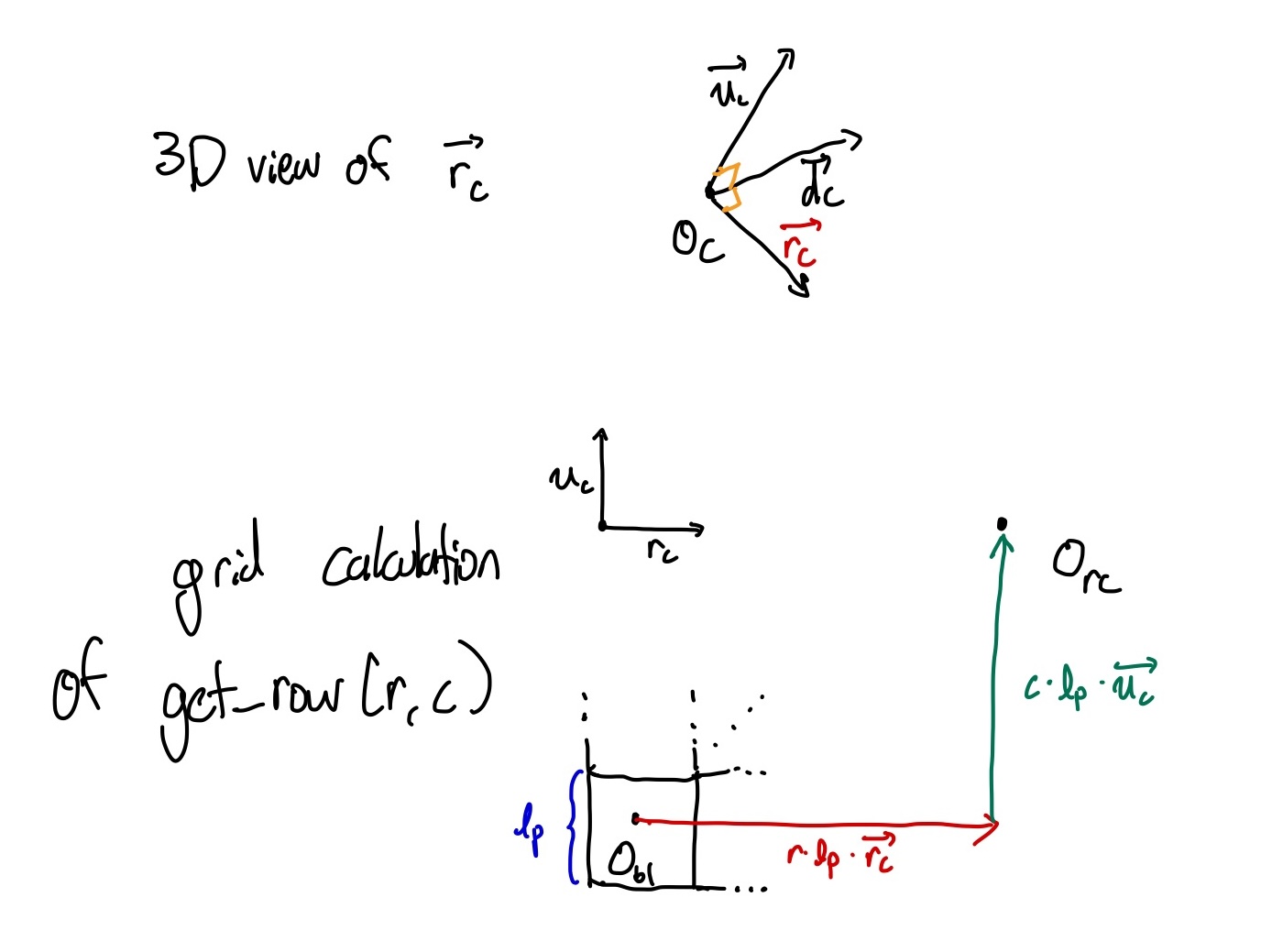
visualizing $\vec{r}_c$ and the pixel ray calculation
With our camera functionality completed, we can move onto the next part: when a ray leaves the camera, it needs to intersect with something in the scene. What could it possibly intersect with?
Introduced Symbols
- $\mathbf{o}_{rc}$: center of pixel $(r,c)$
- $\mathbf{\hat{d}}_p$: direction of a ray pointed at pixel $p$ from the camera origin
- $w$: width of the sensor grid, which is 1 unit from the camera center at its closest point
- $l_p$: side length of a pixel on our grid
- $\vec{r}_c$: the rightward direction on the grid given by $\vec{d}_c \times \vec{u}_c$
- $\mathbf{o}_{bl}$: the position of the center of pixel $(0,0)$ in the bottom left of the sensor
Spheres
but if triangles are made of skin, how are they soldiers? - LL, 2018/2019, D Block Geometry
We will begin with tracing spheres, because they are easy. There is not much intuition here, and we just need to derive an intersection formula. Spheres are defined formally by an origin and radius $(\mathbf{o}_s, r_s).$ The points of the sphere are given by the set of all points that are exactly $r_s$ distance away from the origin $\mathbf{o}_s$.
Thus, to test intersection, we extend a given ray $(\mathbf{o}_r, \vec{d}_r)$ in its direction to see when (if at all) it intersects the sphere $(\mathbf{o}_s, r_s)$:
$$ \left\lVert \left(\mathbf{o}_r + t\vec{d}_r\right) - \mathbf{o}_s\right\rVert = r_s. $$ Manipulating the symbols a little bit, we have
\begin{align*} \left\lVert \left(\mathbf{o}_r + t\vec{d}_r\right) - \mathbf{o}_s\right\rVert = r_s \newline \left(\mathbf{o}_r + t\vec{d}_r - \mathbf{o}_s\right) \cdot \left(\mathbf{o}_r + t\vec{d}_r - \mathbf{o}_s\right)= r_s^2 \newline t^2 \vec{d}_r \cdot \vec{d}_r + 2t \left[\vec{d}_r \cdot (\mathbf{o}_r - \mathbf{o}_s)\right] + (\mathbf{o}_r - \mathbf{o}_s)^2 - r_s^2 = 0. \end{align*}
We can solve this as a quadratic in $t$:
\begin{align*} a = \vec{d}_r \cdot \vec{d}_r \newline b = 2 \vec{d}_r \cdot (\mathbf{o}_r - \mathbf{o}_s) \newline c = (\mathbf{o}_r - \mathbf{o}_s)^2 - r_s^2. \end{align*}
Be sure to check if the determinant is non negative. If it is negative, then there is no intersection. Otherwise, we have at least one solution to $t,$ and we want the smallest positive solution. Note it should be positive because we only care about the forwards direction.
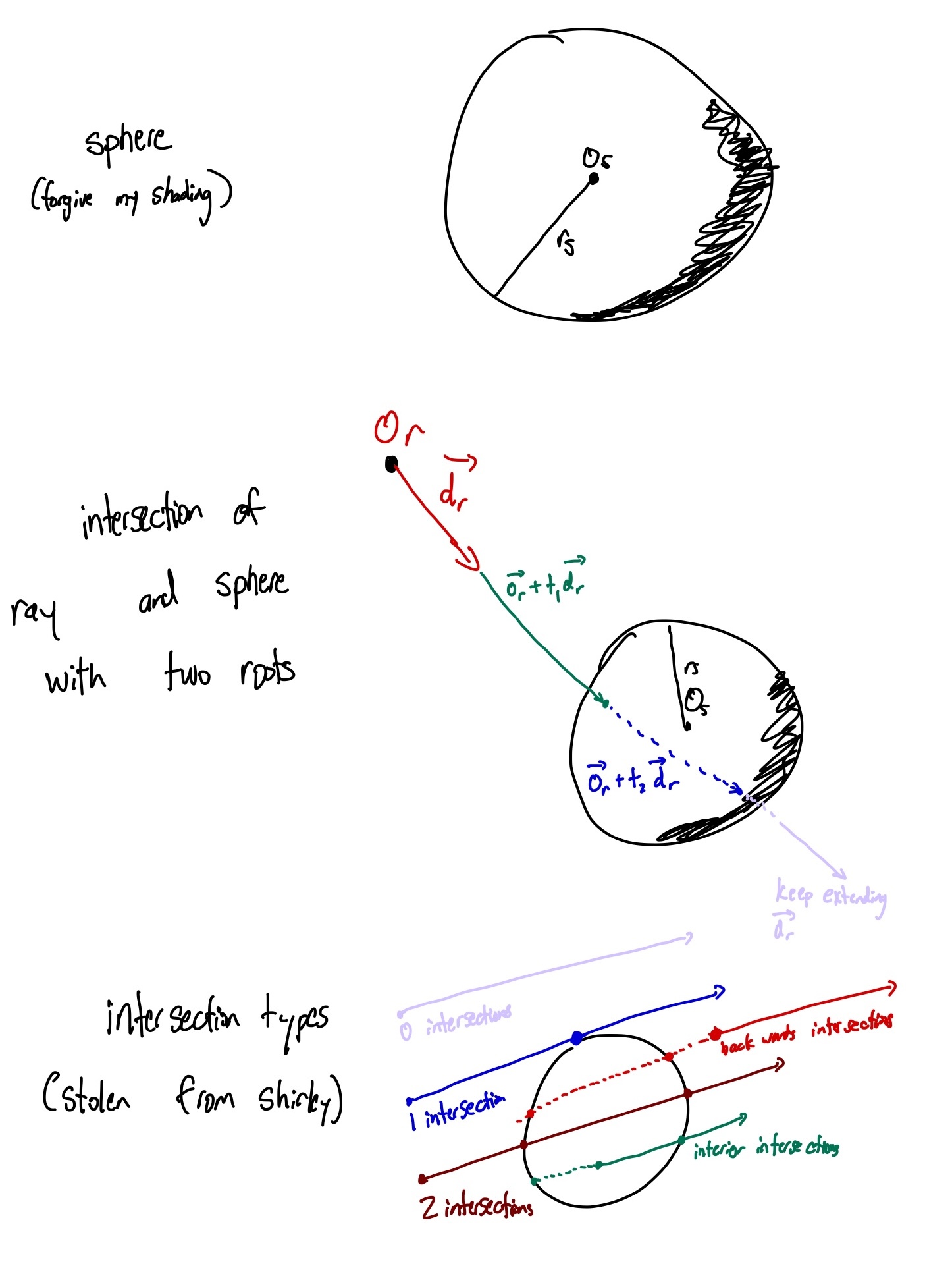
visualizing spheres and the possible intersections with a ray
This gives us a method to check whether or not any given ray intersects a given sphere. We’re ready to trace some rays and intersect them now, but what happens once we intersect a sphere? Find out in the next episode…
Introduced Symbols
- $\mathbf{o}_s$: origin of a sphere
- $r_s$: radius of a sphere
- $\mathbf{o}_r$: variable for origin of a ray
- $d_r$: variable for direction of a ray
Materials
the black lightsaber has got to be made of the strongest stuff - me (paraphrased), 2014
Now with a surface to reflect light off of, we should know how to reflect light off of the materials. Let’s think a little bit about what light bouncing off a surface means.

familiar sights to genz Americans
Consider the image above. We have a few different reflective materials here—on the figure (gogo) we have a shiny silvery coating, with matte yellow and black paint, and we also have a leathery texture underneath that is somewhere between the two. What’s the difference between how these look? Notice how the silvery coating is more sensitive to the directionality of the light from the difference of the left and right sides, and notice how the yellow is much more uniform.
These will roughly be the two materials we’ll be implementing: a soft, matte material, and a shiny, reflective material.
First, let’s describe a diffuse material. A diffuse material does not reflect light in any special way and is not very sensitive to the way light hits it so the light spreads softly and evenly. If we zoom into an intersection surface, we can view this as bouncing the light randomly, so all the incoming light gets averaged into the visible color.
Let’s consider a ray intersecting a diffuse surface. Zooming in, $\vec{\omega_i}$ intersects the surface at point $\mathbf{p}.$ From here, we’ll draw a unit sphere around $\mathbf{p}$, sample that sphere uniformly, and add on the normal, and normalize it. This is a simple way to implement this kind of diffuse, although for a perfectly diffuse material we’ll want to sample it with more rigor.
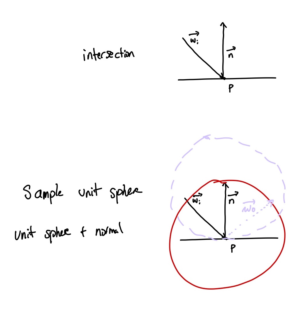
diffuse reflection
Question: Why don’t we sample the hemisphere uniformly? Or rather why do we sample it specifically like this? What’s up with this circle nonsense?
Answer: See the appendix. tw: math. In short, the light is reflected stronger in the direction of the normal, and this sampling method matches a cosine distribution. Thus, we could sample randomly and adjust by the pdf, but this is easier to understand and implement if you don’t think too hard about it (and why would you?). In less technical terms, the more direct the light the stronger its influence, so we want to sample those parts more.
Next, let’s consider a metal material. You can imagine this to be a mirror-like material.
When light intersects a mirror material, it will reflect perfectly across the normal. There’s really not much else to say. Technically, given the intersection point $\mathbf{p}$ and the normal $\vec{n}$, the outgoing ray $\vec{\omega_o}$ will be reflected across the normal which is given by $\vec{\omega}_o = \vec{\omega}_i – 2(\vec{\omega}_i \cdot \vec{n}) \vec{n}$. This is essentially because the “horizontal” part of the incoming ray is the same as the outgoing ray, so we subtract two times the vertical part of the incoming ray relative to the normal.
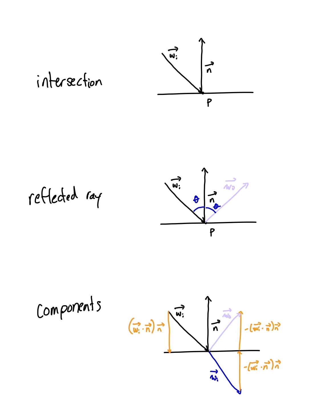
metal reflection
We haven’t talked about colors yet! We want materials to give off colors. At a high level, we’ll simply assign a value $\rho$ to a material that represents the color it reflects. That is, if a ray of light hits a material, $\rho$ will be the amount of light that gets reflected back. For example, blue colored materials will reflect more blue proportional to the other colors.
Introduced Symbols
- $\vec{\omega}_i$: incoming ray
- $\vec{\omega}_o$: outgoing ray
- $\mathbf{p}$: intersection point
- $\vec{n}$: normal ray at a given $\mathbf{p}$
Light
We’ve discussed how to get our rays, how to trace them, and how to bounce them around. But we haven’t really talked about maybe one of the most important part: what color is our damn pixel? Until now, our rays of light have been more or less informationless, where they simply have a start and a direction. If we consider what makes a color up, it’s a spectrum of light of specific frequencies and their intensities. While we won’t discuss this in too much depth and defer to the standard RGB colorspace, there are many different ways to do this and are explained in depth in other resources [pbrt cough cough].
Since we are going for pretty, photorealistic pictures, then we don’t particularly care about units here. We’ll simply use floats in [0,1] to represent our color values with 0 being black, and 1 being the brightest possible. We do allow values above 1, but it simply represents overexposed parts of the image.
We’ll also touch a little bit on gamma correction. Our simulation here will produce ‘absolute’ values of light—that is, we attempt to calculate a numerical value that should be proportional to the number of photons striking the sensor. However, our eyes do not perceive light perfectly proportionally to the intensity, and follows a stronger power curve where most of the intensity is gained at very small values. See here for some better explanations and charts. What this means for our implementation is that we need to adjust the intensity, and typically this means taking things to the $1/2.2$ power.
With the details out of the way, we’ll move into putting them together into code to run and get our pretty pictures.
Implementation
The high level loop of our program will look like the following:
for each pixel on canvas:
    while still intersecting something in scene:
        trace out ray from canvas into scene and get intersection
        accumulate color information
            add color and any emmitted light at this intersection
        generate new ray from the reflection
Note that we send out a single ray here, and as discussed in the materials section this is probabilistic. We can do this a single time, but chances are, it won’t be very close to accuracy. Thus, we’ll take a number of samples and average them to get a better estimate. See appendix for more detail.
Let’s move onto building an implementation piece by piece here in simply C++. The following sections are a high level overview of what’s going on, and each lives in its own file for my implementation. I will include all the code, so if you copy paste the sections it should work [see github!]—this means more code than necessary will exist, but I will do my best to explain my choices. Note that I will be writing comments inline in addition to small explainers before the code, denoted by //!!
vectors impl
vec3.hpp
To do any of our operations, we need a 3 dimensional class. Let’s call it vec3. We’ll also want to define the operations you think you want. Not many annotations going on here because everything is pretty standard.
#pragma once

#include <cmath>

#include “common.hpp”
#include “debug.hpp”

struct vec3 {
  Float x, y, z;
  vec3() : x(0), y(0), z(0) {}
  vec3(Float x_, Float y_, Float z_) : x(x_), y(y_), z(z_) {}
  // the rest should be trivially generated

  //!! used to iterate over all indices for some operation
  Float operator[](int i) const {
    switch (i) {
    case 0:
      return x;
    case 1:
      return y;
    case 2:
      return z;
    }
    [[unlikely]] CERR_WHEN(
        LOG_WARNING, std::format(“Index {} out of bounds on vec3 access”, i));
    // insta crash because this should never happen
    exit(1);
  }
  Float &operator[](int i) {
    switch (i) {
    case 0:
      return x;
    case 1:
      return y;
    case 2:
      return z;
    }
    [[unlikely]] CERR_WHEN(
        LOG_WARNING, std::format(“Index {} out of bounds on vec3 access”, i));
    // insta crash because this should never happen
    exit(1);
  }

  vec3 operator+(const vec3 &v) const {
    vec3 r(*this);
    return r += v;
  }
  vec3 &operator+=(const vec3 &v) {
    x += v.x;
    y += v.y;
    z += v.z;
    return *this;
  }
  vec3 operator-(const vec3 &v) const {
    vec3 r(*this);
    return r -= v;
  }

  vec3 &operator-=(const vec3 &v) {
    x -= v.x;
    y -= v.y;
    z -= v.z;
    return *this;
  }

  vec3 operator*(Float s) const {
    vec3 r(*this);
    return r *= s;
  }
  vec3 &operator*=(Float s) {
    x *= s;
    y *= s;
    z *= s;
    return *this;
  }
  vec3 operator/(Float s) const {
    vec3 r(*this);
    return r /= s;
  }
  vec3 &operator/=(Float s) {
    x /= s;
    y /= s;
    z /= s;
    return *this;
  }
  Float dot(const vec3 &v) const { return x * v.x + y * v.y + z * v.z; }
  vec3 cross(const vec3 &v) const {
    return vec3(y * v.z - z * v.y, z * v.x - x * v.z, x * v.y - y * v.x);
  }

  Float magsq() const { return dot(*this); }
  Float mag() const { return std::sqrt(magsq()); }
  vec3 &normalize() { return *this /= mag(); }

  std::string to_string() const {
    return std::format(“[vec3: ({}, {}, {})]”, x, y, z);
  }
};

inline Float dot(const vec3 &v1, const vec3 &v2) { return v1.dot(v2); }
inline vec3 cross(const vec3 &v1, const vec3 &v2) { return v1.cross(v2); }
spheres impl
shape.hpp
Next, let’s implement spheres. They’ll need a radius and origin as you’d expect, and the intersection is the same as we’ve described above.
#pragma once

#include <variant>

#include “material.hpp”
#include “utils.hpp”
#include “vec3.hpp”

class Sphere {
public:
  Sphere(vec3 center_, Float radius_) : center(center_), radius(radius_) {}
  std::optional<hit> intersect(const vec3 &o, const vec3 &d) const {
    vec3 oc = o - center;
    Float a = dot(d, d);
    Float b = 2 * dot(oc, d);
    Float c = dot(oc, oc) - radius * radius;
    Float x1, x2;
    if (!quadratic(a, b, c, x1, x2)) {
      return std::nullopt;
    }
    // x2 is smaller
    std::optional<Float> t_opt = std::nullopt;
    if (x2 > 0) {
      t_opt = x2;
    } else if (x1 > 0) {
      t_opt = x1;
    }
    if (!t_opt) {
      return std::nullopt;
    }
    Float t = *t_opt;

    //!! described in utils.hpp
    hit h;
    h.t = t;
    h.p = o + d * t;
    h.n = (h.p - center).normalize();
    h.w_i = d;
    return h;
  }

private:
  vec3 center;
  Float radius;
};

//!! variant so we can add triangle later!
using shape = std::variant<Sphere>;

//!! combine to get the aggregate for a full object
struct object {
  shape s;
  material m;
  color emission{};
};
materials impl
material.hpp
#pragma once

#include <variant>

#include “color.hpp”
#include “utils.hpp”

struct scatter_out {
  color attenuation;
  vec3 new_direction;
};
class Lambertian {
public:
  Lambertian(color albedo) : albedo(albedo) {}
  scatter_out scatter(const hit &h, rng &r) const {
    vec3 new_direction = random_unit_vector(r) + h.n;
    return {albedo, new_direction.normalize()};
  }

private:
  //!! Technically this shouldn’t be called albedo, see appendix for more.
  color albedo;
};

class Metal {
public:
  Metal(color albedo) : albedo(albedo) {}
  scatter_out scatter(const hit &h, rng &r) const {
    vec3 new_direction = h.w_i - h.n * dot(h.w_i, h.n) * 2;
    return {albedo, new_direction};
  }

private:
  color albedo;
};

//!! if we add triangles or other shapes, we’d also have to add it here!
using material = std::variant<Lambertian, Metal>;
cameras impl
camera.hpp
Our camera implementation deviates a little bit from what we’ve described. Since we might not want to bake the height/width into the camera itself, we’ll allow that to be a option to initialize the camera for a scene for different renders. Otherwise, the init function implements what we covered.
//!! I use this pattern maybe more than I should
//!! it lets me effectively give named arguments to a constructor!
struct camera_options {
  vec3 origin, direction, up;
  double fov;
};
class Camera {
public:
  Camera(camera_options co)
      : origin(co.origin), direction(co.direction), up(co.up), fov(co.fov) {
    right = cross(direction, up).normalize();
    up.normalize();
    direction.normalize();
  }
  void init(int height, int width) {
    double w = 2 * std::atan(fov / 2.0);
    lp = w / width;
    bl = origin + direction - (right * lp * width / 2.0) -
         (up * lp * height / 2.0);
  }

  vec3 get_ray(int row, int column, rng &r) const {
    return (bl + (right * lp * (column + r.random_float(-0.5, 0.5))) +
            (up * lp * (row + r.random_float(-0.5, 0.5))) - origin)
        .normalize();
  }
  vec3 get_origin() const { return origin; }

private:
  vec3 origin, direction, up, right, bl;
  double fov, lp;
};
lights impl
color.hpp
We’ll need to implement the pixel/color struct as well containing our RGB values. For the scope of this renderer, we can more or less use the vec3 skeleton we’ve already built because we’ll be using the operations it provides.
#pragma once

#include “common.hpp”
#include “vec3.hpp”

struct color : public vec3 {
  //!! bring constructors into scope
  using vec3::vec3;
  //!! maybe do this in vec3 for uniformity, but it would be
  //!! nice to get aliases like using float r = this->x; or something
  Float &r() { return this->x; }
  Float r() const { return this->x; }
  Float &g() { return this->y; }
  Float g() const { return this->y; }
  Float &b() { return this->z; }
  Float b() const { return this->z; }

  //!! note these are not defined in vec3!
  // element-wise multiplication
  color &operator*=(const color &o) {
    this->r() *= o.r();
    this->g() *= o.g();
    this->b() *= o.b();
    return *this;
  }
  color operator*(const color &o) {
    color t(*this);
    return t *= o;
  }
};
main impl
render.cpp
the meat of the program. this function is called repeatedly to calculate the color of any given pixel.
#include “render.hpp”
#include “scene.hpp”

color integrate(const Scene &s, const render_options &ro, vec3 o, vec3 d,
                rng &r) {
  color result{};
  color throughput{1, 1, 1};

  for (int i = 0; i < ro.bounces; i++) {
    auto hit_opt = s.intersect(o, d);
    if (!hit_opt) {
      // empty!
      result += throughput * s.background;
      break;
    }
    // we have a hit!
    auto hit = *hit_opt;

    result += throughput * hit.obj->emission;

    auto material = hit.obj->m;
    scatter_out s =
        std::visit([&](auto &&m) { return m.scatter(hit, r); }, material);

    throughput *= s.attenuation;

    o = hit.p;
    d = s.new_direction;

    if (i > ro.rr_depth) {
      //!! choosing a p for russian roulette
      //!! I honestly forget where this heuristic comes from
      // this should be dependent on throughput
      // this seems expensive? invokes a sqrt...
      Float q = std::max(0.05, 1 - throughput.mag() * 0.33333);
      if (r.random_float() < q)
        break;
      throughput /= (1 - q);
    }
  }

  return result;
}
scene impl
scene.hpp
The scene is where everything will live, so it needs all the objects and cameras. We’ll also put the big rendering loop that we discussed previous around here. One big piece of functionality Scene needs to implement is hit testing! We can defer the individual object hit testing to the object itself, but the Scene is responsible for finding the first one. We do this simply by linearly searching the entire scene because our ray tracer is dead simple. However, as scenes become more complex, a BVH or space partitioning tree of some sort is usually used to speed up the testing significantly [in fact, to my knowledge the RT cores on a RTX enabled GPU are simply ASICS for BVH traversal!].
Here’s a free class on multithreading: we use OpenMP, which gives us a simple interface to do multithreading over loops. We won’t worry about thread safety because we’ll partition the work such that no inter-thread communication is necessary. Thus, we can take our scene loop and throw a #pragma over it and let OpenMP take care of the work.
OpenMP basically “flattens” this loop and each iteration it assigns it to a thread, so if our work between every iteration is very small whereas we have many iterations, it’d be fair to be concerned about scheduling overhead. We can tile the work so that each iteration of the inner loop is really a 16x16 tile, although this isn’t really all that helpful (overhead seems to be less than 5%). But we’re keeping it anyways because it makes it feel more proper, and deeper, more nested loops is always funny (I think my personal best is 8).
#pragma once

#include <omp.h>

#include “camera.hpp”
#include “color.hpp”
#include “common.hpp”
#include “render.hpp”
#include “shape.hpp”

//!! essentially constructor information
struct scene_options {
  Camera cam;
  std::vector<object> objects;
  color background;
};
//!! options for rendering an image
struct render_options {
  int height;
  int width;
  int samples;
  int bounces;
  Float gamma;
  int threads = 1;
  int tile_size = 16;
  int rr_depth = 3;
};

class Scene {
public:
  Scene(const scene_options &so) : camera(so.cam), background(so.background) {
    objects.reserve(so.objects.size());
    for (const auto &obj : so.objects) {
      add_object(obj);
    }
  }

  void add_objects(const std::vector<object> &objs) {
    objects.insert(objects.end(), objs.begin(), objs.end());
  }
  void add_object(const object &obj) { objects.push_back(obj); }
  void add_object(object &&obj) { objects.emplace_back(obj); }

  std::optional<hit> intersect(const vec3 &o, const vec3 &d) const {
    std::optional<hit> hit_opt = std::nullopt;
    //!! we loop through all objects, and check if it is the closest
    //!! intersection so far. if so, take it, otherwise, move on.
    for (const auto &obj : objects) {
      auto hit_opt_ =
          std::visit([&](auto &&arg) { return arg.intersect(o, d); }, obj.s);
      if (!hit_opt_)
        continue;
      if (!hit_opt) {
        hit_opt = *hit_opt_;
        hit_opt->obj = &obj;
      } else {
        if (hit_opt_->t > hit_opt_->t) {
          hit_opt = *hit_opt_;
          hit_opt->obj = &obj;
        }
      }
    }
    return hit_opt;
  }

  image render(const render_options &ro) {
    camera.init(ro.height, ro.width);

    image result;
    result.data.resize(ro.height * ro.width);
    result.height = ro.height;
    result.width = ro.width;

    //!! each thread will need its own independent rng engine
    //!! since the internals of an rng engine have state, we’d need
    //!! synchronization otherwise which is pointless because we can simply
    //!! provide each thread with its own unique engine
    std::vector<rng> rngs;
    int n_threads = 1;
#ifdef _OPENMP
    omp_set_num_threads(ro.threads);
    n_threads = ro.threads;
#endif
    std::random_device rd{};
    for (int i = 0; i < n_threads; i++) {
      rngs.emplace_back(rng{rd()});
    }

    //!! magic macro! #pragma omp declares the OpenMP macro
    //!! parallel for should be fairly straightforward, collapse(2)
    //!! tells the compiler how many levels to “flatten” and allow multithreading for.
    //!! here, we don’t want the inner tiling loops to be flattened,
    //!! so we only collapse 2
    //!! schedule(dynamic) tells the OpenMP scheduler that it can schedule
    //!! them on demand, rather than statically assigning
    //!! job i to [i % num_threads] for example. this is important in
    //!! ray tracing because we can have tiles that take much longer
    //!! to render where there are lots of bounces and objects, and
    //!! blank spots where a ray misses and we only pick up a
    //!! background color. Thus, each tile has an unbalanced
    //!! amount of work so we should schedule them at runtime.
#pragma omp parallel for collapse(2) schedule(dynamic)
    for (int r = 0; r < ro.height; r += ro.tile_size) {
      for (int c = 0; c < ro.width; c += ro.tile_size) {

        int rng_idx = 0;
#ifdef _OPENMP
        rng_idx = omp_get_thread_num();
#endif

        //!! we tile the appropriate amount, and this becomes our inner loop
        for (int rr = r; rr < std::min(r + ro.tile_size, ro.height); rr++) {
          for (int cc = c; cc < std::min(c + ro.tile_size, ro.width); cc++) {
            color pixel_color{};
            //!! for each sample, we extend a ray into the scene and trace
            for (int s = 0; s < ro.samples; s++) {
              vec3 co = camera.get_origin();

              vec3 dir = camera.get_ray(rr, cc, rngs[rng_idx]);
              pixel_color += integrate(*this, ro, co, dir, rngs[rng_idx]);
            }
            // postprocess
            //!! As a Monte-Carlo program, we take the average color
            pixel_color /= ro.samples;

            //!! gamma correction
            for (int idx = 0; idx < 3; idx++)
              if (pixel_color[idx] > 0.0)
                pixel_color[idx] = std::pow(pixel_color[idx], 1.0 / ro.gamma);

            result.data[rr * ro.width + cc] = pixel_color;
          }
        }
      }
    }

    return result;
  }
  const std::vector<object> &get_objects() const { return objects; }
  const color background;

private:
  Camera camera;
  std::vector<object> objects;
};
misc impl
There’s a handful of things we haven’t covered, and it’ll all be thrown into a common file until it finds a better home. This includes an aggregate for an intersection, an image aggregate to sling the data around, a random number generator and the affiliated functions, a function for printing .ppm images, and the fabled quadratic function.
#pragma once

#include <algorithm>
#include <cmath>
#include <iostream>
#include <numbers>
#include <random>
#include <vector>

#include “color.hpp”
#include “vec3.hpp”

struct object;

//!! this probably is not a great place for this haha
//!! because we need the forward declaration to make this work!
struct hit {
  Float t;
  vec3 p, n, w_i;
  const object *obj;
};

//!! super simple image struct to help us sling pixels around
struct image {
  int width, height;
  // row major: (r, c) = row * width + c
  std::vector<color> data;
};

//!! as a monte carlo program, we need a source of randomness!
//!! We use std::mt19937 here but many implementations use the
//!! pcg family for good quality and fast random numbers
//!! there’s quite some theory here, and generally it’s better to have
//!! even coverage than truly random coverage so some opt to use
//!! low discrepency sequences (especially on camera sampling!)
class rng_std {
public:
  rng_std() : m_rng(0) {}
  rng_std(uint64_t seed) : m_rng(seed) {}
  Float random_float(Float lo = 0.0, Float hi = 1.0) {
    std::uniform_real_distribution<Float> dist(lo, hi);
    return dist(m_rng);
  }

  static rng_std &get() {
    static rng_std instance;
    return instance;
  }

private:
  std::mt19937 m_rng;
};
using rng = rng_std;

//!! inline so we can keep our .hpp warning free :)
//!! this is one way to uniformly sample a unit vector
//!! again sampling is difficult and I haven’t thought about
//!! it enough to be confident enough to write about it.
//!! No, picking a random theta and phi does not work (poles will be oversaturated).
inline vec3 random_unit_vector(rng &r) {
  Float u = r.random_float();
  Float v = r.random_float();
  Float theta = 2 * std::numbers::pi * u;
  Float phi = std::acos(2 * v - 1);

  return vec3{std::sin(phi) * std::cos(theta), std::sin(phi) * std::sin(theta),
              std::cos(phi)};
}

// scales f to [lo, hi], on a scale from [0, 1]
template <class Float, class T> T scale(Float f, T lo, T hi) {
  T range = hi - lo;

  f = std::clamp(f, (Float)0, (Float)1);
  return (T)(f * range);
}

//!! writing images to ppm.
//!! header is magic number P3 for ascii rgb, width and height are self
//!! explanatory, 255 is the max value (1 byte)
template <class Stream> Stream &write_ppm(Stream &file, const image &im) {
  file << “P3\n”
       << im.width << " " << im.height << “\n”
       << “255\n”;

  // the way we do this it’s upside down since (0,0) is the bottom left
  // PPM goes top down
  for (int row = im.height - 1; row >= 0; row–) {
    for (int c = 0; c < im.width; c++) {
      const color &pix = im.data[row * im.width + c];
      int r = scale(pix.x, 0, 255);
      int g = scale(pix.y, 0, 255);
      int b = scale(pix.z, 0, 255);

      file << r << " " << g << " " << b << “\n”;
    }
  }
  return file;
};

//!! yeah the comment below means I didn’t think about this very much
//!! I believe there are numerical stability issues so there are better
//!! ways to do this, but this seems to work well enough
//!! attribute for fun :) but the label tells gnu that this code should be optimized more
// this is not optimized but issok
[[gnu::hot]] inline bool quadratic(Float a, Float b, Float c, Float &x1,
                                   Float &x2) {
  // first use standard formula
  Float d = b * b - 4 * a * c;
  if (d < 0) {
    return false;
  }
  if (d == 0) {
    x1 = x2 = -b / (2 * a);
    return true;
  }
  x1 = (-b + std::sqrt(d)) / (2 * a);
  x2 = (-b - std::sqrt(d)) / (2 * a);
  return true;
}
compiling & usage
main.cpp
Question: How do we compile this code? Where’s my makefile?
Answer: I don’t have one. To compile the code, simply use g++ -std=c++23 -O3 main.cpp render.cpp and any other files you add. Alternatively, I used g++ -std=c++23 -O3 *.cpp since I only have those two .cpp files with one main function. Why 23? I don’t use 23 features, but I get issues with the standard library compiling with 20, so go figure [specifically with std::format and std::optional—I understand the issues with std::format but why optional? couldn’t tell you].
Question: How do I write a main.cpp to render my own scene?
Answer: You’ll have to do it by hand. Because our ray tracer is enormously simple, it’ll be hard to render anything substantial but spheres are already pretty cool [challenge: implement triangles and you can import .obj and other file types!]. One can look at main.cpp for more reference, and you’re free to modify the constructors/functions as you see fit for convenience but the name of the game is roughly to:
- construct objects
- construct camera
- construct scene
- render our scene
We construct objects by combining a geometry and a material, a camera by providing the necessary information covered in cameras, a scene by giving a list of objects and a camera [plus a backdrop!], and finally we can render by providing some dimensions and settings. We’ll get our output as a pixel grid, and hopefully we want to view it so we can save it to a file.
#include <iostream>

#include “color.hpp”
#include “debug.hpp”
#include “scene.hpp”
#include “utils.hpp”

int main() {
  //!! Creating our objects. Recall sphere constructs with (center, radius), whereas
  //!! lambertian constructs with (color)

  Sphere s{vec3{0, 1, 0}, 0.5};
  Lambertian l{color{1, 0.2, 0.2}};
  Sphere s2{vec3{0.4, 0.8, -0.5}, 0.2};
  Lambertian l2{color{0.2, 0.8, 0.5}};
  Sphere s3{vec3{-0.4, 0.8, 0.5}, 0.2};
  Metal l3{color{0.2, 0.3, 0.9}};

  //!! Combining a geometry and a material to get an object. Objects can be emissive,
  //!! but we omit this to indicate no emission.
  object o{s, l};
  object o2{s2, l2};
  object o3{s3, l3};

  //!! options for the camera.
  camera_options co{.origin = vec3{0, -1, 0},
                    .direction = vec3{0, 1, 0},
                    .up = vec3{0, 0, 1},
                    .fov = 70};
  Camera c{co};

  //!! options for the scene.
  scene_options so{
      .cam = c, .objects = {o, o2, o3}, .background = color{0.5, 0.7, 1}};
  Scene sc{so};

  //!! options for the render. Again, we input these as parameters
  //!! to make it easy to render the same scene in different ways.
  render_options ro{.height = 2000,
                    .width = 3000,
                    .samples = 1000,
                    .bounces = 7,
                    .gamma = 2.2,
                    .threads = 7};
  auto img = sc.render(ro);

  //!! write the image out
  std::ofstream of(“test.ppm”);
  write_ppm(of, img);
}
There’s at least one file I don’t cover here, but there’s no functionality missing here. Check the github.
The End
Ok I didn’t read it. what’s the tldr?
light trace go brrrr.
Appendix A
symbol soup for sale!
We are really trying to solve the rendering equation here.
Veach does a better job than me formalizing this (obviously) but we are trying to find the incoming light at a given point and direction. We’ll define a few terms here:
- $L_i(\mathbf{p}, \omega)$: incoming light at point $\mathbf{p}$ in direction $\vec{\omega}$ pointing towards $\mathbf{p}$
- $L_o(\mathbf{p}, \omega)$: outgoing light from point $\mathbf{p}$ in direction $\vec{\omega}$ pointing away from $\mathbf{p}$
- $L_e(\mathbf{p}, \omega)$: emitted light from point $\mathbf{p}$ in direction $\vec{\omega}$ pointing away from $\mathbf{p}$
- $\Omega$: Hemisphere in the direction of the normal
- $f(\mathbf{p}, \vec{\omega}_i, \vec{\omega}_o)$: bidirectional reflectance distribution function (BRDF), which gives a “distribution” over the hemisphere in terms of light incoming from $\vec{\omega}_i$ and how it reflects in any given direction $\vec{\omega}_o$ at a point $\mathbf{p}$. There are many other distribution functions which is why you’ll see BxDF pop up—we only care about BRDF’s for the scope of this appendix. BTDF (transmission) is used for transparent objects, and BSDF (scattering) combines the two.
$L_i$ and $L_o$ are very closely related functions! In fact, we can define them in terms of eachother: $$L_o(\mathbf{p}, \vec{\omega}_o) = \int_\Omega f(\mathbf{p},\vec{\omega}_i, \vec{\omega}_o) L_i(\mathbf{p}, \vec{\omega}_i) | \vec{\omega}_i \cdot \vec{n} | d\vec{\omega}_i$$ $$L_i(\mathbf{p}, \vec{\omega}_i) = L_o(\mathbf{p}’, \vec{\omega}_i) + L_e(\mathbf{p}’, \vec{\omega}_i)$$ where $\mathbf{p}’$ is the nearest intersection between the ray $(\mathbf{p}, -\vec{\omega}_i)$ and the scene. Note that it’s negative because it’s an incoming direction.
The one term we haven’t discussed is the $| \vec{\omega}_i \cdot \vec{n}|$ term. This is the incident angle term, and the short version is that if light hits at an angle, it is more spread out compared to being fully concentrated at the point of intersection. The dot product gives us the cosine of the smallest angle between the two vectors, so this will weigh things by how directly they strike the intersection point.
Putting everything together, we have that the outgoing light at a point $\mathbf{p}$ is the the contribution of all the light incoming over the hemisphere, factored by the BRDF and the incident angle.
There are two questions I’d like to answer in this section that are relevant to the post.
- How does this equation show up in the implementation
- How does our sampling solve this equation
We’ll tackle the first point first. Notice how our renderer effectively implements $L_i$, except our direction points the other way We trace a ray into the scene repeatedly, and get an intersection point, where we ask what $L_o$ at that point is. Our implementation function integrate is iterative, but we can actually derive it from a fully recursive form:
$$ \begin{align*} L_i(\mathbf{p}, \vec{\omega}_i) = L_o(\mathbf{p}’, \vec{\omega}_i) + L_e(\mathbf{p}’, \vec{\omega}_i) = \int_\Omega f(\mathbf{p}’,\vec{\omega}_i, \vec{\omega}) L_i(\mathbf{p}’, \vec{\omega}) | \vec{\omega} \cdot \vec{n} | d\vec{\omega} + L_e(\mathbf{p}’, \vec{\omega}_i) \newline =\int_\Omega \left[L_o(\mathbf{p}’’, \vec{\omega}) + L_e(\mathbf{p}’’, \vec{\omega})\right]f(\mathbf{p}’, \vec{\omega_i}, \vec{\omega}) | \vec{\omega} \cdot \vec{n} | d\vec{\omega} + L_e(\mathbf{p}’, \vec{\omega}_i) \text{ (by expanding } L_i \text{)} \end{align*} $$ We’ll expand this one more time just to see, but this does go on infinitely. We’ll let $f(\mathbf{p}’, \vec{\omega_i}, \vec{\omega}) = \alpha$ and $| \vec{\omega} \cdot \vec{n} | = \beta$ to save space.
$$ \begin{align*} =\int_\Omega \left(\left[ \alpha\beta \cdot \int_{\Omega’}f(\mathbf{p}’’, \vec{\omega}’, \vec{\omega})L_i(\mathbf{p}’’, \vec{\omega}’) |\vec{\omega}’ \cdot \vec{n}| d\vec{\omega}’ \right] + \alpha\beta L_e(\mathbf{p}’’, \vec{\omega}) d\vec{\omega}\right) + L_e(\mathbf{p}’, \vec{\omega}_i) \end{align*} $$
Some things to notice - we want to pick up these $\alpha \beta$ terms as we go, and if you look towards the right hand side of the equation we are accumulating the $L_e$ at different hit points throughout, while continuously mulitplying by $\alpha \beta.$ A fully [tail :)] recursive way to do this would be to have a function akin to
L_i(p,w):
    q <- get an intersection point
    get material
    d <- sample a new direction
    return alpha * beta * L_i(q,-d) + L_e(q,w)
We can avoid the overhead of recursion and reason about this better by doing a loop:
L_i(p,w):
    throughput <- 1
    acc <- no color
    for # of bounces:
        q <- get an intersection point
        get material
        d <- sample a new direction

        acc += L_e(q,w) * throughput
        throughput *= alpha * beta
        p <- q
        w <- d
    return acc
Note that this isn’t fully equivalent, because in the recursive version we didn’t specify how many bounces to go. Technically, it should be infinite, but in most scenes the throughput will fall off very quickly, so setting the maximum number of bounces at 10 is more than reasonable. This does bias our tracer! One way to get around this is through russian-roulette sampling: we want to have the chance of going to infinite bounces, but since most contributions at that point are useless, we’ll do some probabilistic culling.
Our goal is to get an estimator for the incoming light so that we can take samples for it that will converge to its true value, but it can be difficult to calculate—in our case, the ray tracing integral goes on forever [infinte dimensional] and thus it’s impossible to calculate all the way out. We’d like a method to be able to calculate this in an unbiased manner, as one can imagine if we cut everything off after some point this is not guaranteed to give us accurate results. For instance, if we have a box with many mirrors, each bounce does in fact contribute more information, so if we stop at 7 vs 8 bounces, this would visually make a difference. Thus, implementing this with a max number of bounces technically will not produce a correct answer, even if we take infinite samples, meaning our estimator here is biased.
To see how to unbias it [in theory], let’s take a step back and consider an arbitrary function $f(x)$. We’ll modify it in the following way, for a random $r$ chosen from a uniform $[0,1]$ distribution, and a parameter $p \in [0,1]$. $$ f’(x,r) = \begin{cases} \frac{f(x)}{p}, r < p \newline 0, r > p \end{cases} $$ If we consider the expected value of $f’$ with respect to this new parameter $r,$ we have $$\mathbb{E}[f’] = p \cdot \frac{f(x)}{p} + (1-p) \cdot 0 = f(x)$$ so we see that $f’$ in expectation will be equivalent to $f,$ and that in theory, could replace $f$ and we could let it go on forever. Since at each step it has a probability of terminating $p,$ the probability that this process continues shrinks exponentially, so we have effectively bounded our computation time while getting an unbiased answer [but we’ll bound the max bounces anyways in practice]. You can find more details about this in PBRT and also Veach.
This concludes our answer to the first question—we are trying to solve the rendering equation, this shows up in our function that does the bounces, and this is also why it is called integrate.
For the second question, one might have noticed we waved our hands a little bit [more than I should have] when looking at the integral and the implementation. There’s no $\beta$ term in the implementation! This is not a mistake. We do not account for the $\beta$ term when we trace our rays on purpose. In a full fledged ray tracer, we would, but since we are implementing a simple one here, we can implement our integrator to avoid it.
Let’s first revisit what it means to be a diffuse, or otherwise known as Lambertian, material. In the materials section, I simply said it was a soft material that bounces light randomly. To put it more formally, a diffuse material reflects uniformly over the hemisphere, irrespective of incoming angle. Thus, we should really be sampling the hemisphere uniformly shouldn’t we?
We could do this, but let’s recall how Monte Carlo integration works.
The basic example is to integrate some [integrable] function $f : \mathbb{R} \to \mathbb{R}$ over some interval $[a,b]$. We have the estimate
$$ \int_a^b f(x)dx \approx \frac{b-a}{N} \sum_{i=1}^N f(x_i) $$ assuming $x_i$ are iid. drawn uniformly from $[a,b].$
If we take the expected value on the RHS, we have $$ \begin{align*} \mathbb{E}\left[\frac{b-a}{N} \sum_{i=1}^N f(x_i)\right] = \frac{b-a}{N} \sum_{i=1}^N \mathbb{E}[f(x_i)] \newline = (b-a) \int_a^b \frac{f(x)}{b-a}dx = \int_a^b f(x)dx \end{align*} $$ as desired.
More generally, we can draw samples from an arbitrary distribution $p$ and equally take the estimate
$$ \int_a^b f(x)dx \approx \frac{1}{N} \sum_{i=1}^N \frac{f(x_i)}{p(x_i)}. $$
with $x_i$ drawn in proportion to $p$. Then, expanding the RHS again we have
$$ \begin{align*} \mathbb{E}\left[\frac{1}{N} \sum_{i=1}^N \frac{f(x_i)}{p(x_i)}\right] = \frac{1}{N} \sum_{i=1}^N \mathbb{E}\left[\frac{f(x_i)}{p(x_i)}\right] \newline = \int_a^b \frac{f(x)}{p(x)}p(x)dx = \int_a^b f(x)dx \end{align*} $$ once again, where the expected value operator is now with respect to $p$.
Note that this now works with an arbitrary domain, and not just the interval! Now, if we know something about this function $f,$ and that it takes on large values around some subset of the domain, and near zero elsewhere, it’ll probably be better worth our time to focus on that portion with a larger contribution, and then adjust by the probability of our draw.
We’ll do the same thing with the rendering equation—we don’t necessarily need to match a distribution, but we’ll hit out the incident angle here.
Let’s see the vanilla sampling here, where we draw from the unit hemisphere uniformly instead of the weighted way we implement.
$$ \begin{align*} L_i(\mathbf{p}, \vec{\omega}_i) = L_o(\mathbf{p}’, \vec{\omega}_i) + L_e(\mathbf{p}’, \vec{\omega}_i) = \int_\Omega f(\mathbf{p}’,\vec{\omega}_i, \vec{\omega}) L_i(\mathbf{p}’, \vec{\omega}) | \vec{\omega} \cdot \vec{n} | d\vec{\omega} + L_e(\mathbf{p}’, \vec{\omega}_i) \newline \approx L_e(\mathbf{p}’, \vec{\omega}_k)+ \frac{1}{N} \sum_{k=1}^N 2\pi \cdot f(\mathbf{p}’, \vec{\omega}_i, \vec{\omega}_k)L_i(\mathbf{p},\vec{\omega}_k) | \vec{\omega}_k \cdot \vec{n} | \end{align*} $$ assuming we draw $\vec{\omega}_k$ from a uniform distribution over $\Omega$ [hemisphere] with a pdf $p(x) = \frac{1}{2\pi}$. Let’s find the expected value. We’ll ignore the emission term because it’s constant and takes up space.
$$ \begin{align*} \mathbb{E}\left[ \frac{1}{N} \sum_{k=1}^N 2 \pi \cdot f(\mathbf{p}’, \vec{\omega}_i, \vec{\omega}_k)L_i(\mathbf{p},\vec{\omega}_k) | \vec{\omega}_k \cdot \vec{n} |\right] \newline = \frac{1}{N} \sum_{k=1}^N \mathbb{E} \left[2\pi \cdot f(\mathbf{p}’, \vec{\omega}_i, \vec{\omega}_k)L_i(\mathbf{p},\vec{\omega}_k) | \vec{\omega}_k \cdot \vec{n} |\right] \newline = 2 \pi \int_\Omega f(\mathbf{p}’, \vec{\omega}_i, \vec{\omega}) L_i(\mathbf{p}’, \vec{\omega}) | \vec{\omega} \cdot \vec{n} | p(\vec{\omega}) d\vec{\omega} \newline = \int_\Omega f(\mathbf{p}’, \vec{\omega}_i, \vec{\omega}) L_i(\mathbf{p}’, \vec{\omega}) | \vec{\omega} \cdot \vec{n} | d\vec{\omega} \end{align*} $$ as $p(\vec{\omega}) = \frac{1}{2\pi}$, and they cancel out exactly as we hope. However, let’s try sampling from a a cosine distribution here. The distribution of a cosine weighted hemisphere is $p(\vec{\omega}) = \frac{\cos(\theta)}{\pi},$ where $\pi$ is a normalizing term for the distribution.
$$ \begin{align*} \mathbb{E}\left[\frac{1}{N} \sum_{k=1}^N \frac{f(\mathbf{p}’, \vec{\omega}_i, \vec{\omega}_k)L_i(\mathbf{p},\vec{\omega}_k) | \vec{\omega}_k \cdot \vec{n} |}{\frac{\cos(\theta)}{\pi}}\right] \end{align*}. $$ But $\cos(\theta) = | \vec{\omega} \cdot \vec{n} |$—so let’s cancel here! $$ \begin{align*} \mathbb{E}\left[\frac{1}{N} \sum_{k=1}^N \frac{f(\mathbf{p}’, \vec{\omega}_i, \vec{\omega}_k)L_i(\mathbf{p},\vec{\omega}_k) \cos(\theta)}{\frac{\cos(\theta)}{\pi}}\right] \newline = \pi \cdot \int_\Omega f(\mathbf{p}’, \vec{\omega}_i, \vec{\omega})L_i(\mathbf{p},\vec{\omega}) p(\vec{\omega}) d\vec{\omega} \newline = \pi \cdot \int_\Omega f(\mathbf{p}’, \vec{\omega}_i, \vec{\omega})L_i(\mathbf{p},\vec{\omega}) \frac{\cos(\theta)}{\pi} d\vec{\omega} \end{align*} $$ which as you imagine, will cancel out. However, notice that the terms cancel before we even apply the integral! So we’re left simply with $$ \mathbb{E}\left[\frac{1}{N} \sum_{k=1}^N \pi \cdot f(\mathbf{p}’, \vec{\omega}_i, \vec{\omega}_k)L_i(\mathbf{p},\vec{\omega}_k) \right] = \int_\Omega f(\mathbf{p}’, \vec{\omega}_i, \vec{\omega})L_i(\mathbf{p},\vec{\omega}) | \vec{\omega} \cdot \vec{n} | d\vec{\omega}.$$
If you’re following along, this means that we don’t have to explicitly factor in that $\cos$ term in the integral! If we sample our Lambertian from a cosine distribution, then it’ll be encoded in the distribution. We deal with the $\pi$ factor by dividing by $\pi$ in the BRDF. We don’t really implement a full fledged BRDF, and only look at the albedo, but in a proper implementation the BRDF does factor this in.
To see this formally, if we consider a fixed wavelength of light, our albedo $\rho \in [0,1]$ is the proportion of light reflected by the material. We then want $$ \int_\Omega f(\mathbf{p}, \vec{\omega}_i, \vec{\omega}) |\vec{\omega} \cdot \vec{n} | d\vec{\omega} = \rho $$ because this gives us the total amount of light reflected from a fixed incoming, which is precisely what our albedo represents. Let’s call the $f(\mathbf{p}, \vec{\omega}_i, \vec{\omega}) = c$ because it’s constant, and we see that $$ c \int_\Omega |\vec{\omega} \cdot \vec{n} | d\vec{\omega} = c \pi, $$ and we see that $c = \frac{\rho}{\pi}.$ If we plug this into our estimator, we are left with $$ \int_\Omega f(\mathbf{p}’, \vec{\omega}_i, \vec{\omega})L_i(\mathbf{p},\vec{\omega}) | \vec{\omega} \cdot \vec{n} | d\vec{\omega} = \mathbb{E}\left[\rho L_i(\mathbf{p},\vec{\omega}) \right] \approx \frac{1}{N} \sum_{k=1}^N \rho L_i(\mathbf{p}, \vec{\omega}_k)$$ which is the form of our ray tracer—we only accumulate albedo!
Now we are imagining a world where we only have a Lambertian. So close to the real world, where we have a Lambertian and a metal material. But still so far. Not to worry. Let’s think a little harder. The Rendering Equation is used when we want to factor in light from all directions, but in metals, light is perfectly reflected across the normal, so there is no integral needed! So no cosine term! No conservation of energy violated, no work needed to be done. win win.
That concludes our answer to the second question. Our sampler solves this equation by sampling the Lambertian in a cosine-distributed manner, which gives us the correct solution to the Rendering Equation without any adjustments, while our metal material doesn’t need to worry about the equation at all.
[TODO: references lol]